Understanding Process Time Variation
If a factory doesn't make rate, or otherwise underperforms, the problem is often with the variation in process times — and insufficient capacity and inventory to compensate for it. If a process takes longer than the mean, the workstation is blocked, downstream equipment may run into starvation and underutilization. Likewise, a shorter-than-usual process time can lead to starvation upstream and blocking downstream.
If not enough capacity and inventory is available — both can compensate — the system may not be able to meet production rate targets.
There are few things that are so often misunderstood as process time variation. Many factory managers, even industrial engineers, struggle to consider the significant impact of process time variation, with serious consequences for production system performance.
Read a related case study: how instructions to stop beating champion times saved $6 m/yr: read more ...
Here are just some of the biggest myths:
Common Myths
Myth 1: "If processes are faster at least as much as they take longer, the effects cancel each other out."
False. Variation leads to unpredictable arrival rates down the line, which lead to empty machines and large buffers, i.e. a reduction in effective capacity.
Myth 2: "Automated processes do not contribute to variation."
Does part geometry or quality affect process times? Is a human worker still required for loading or unloading? Can an automated machine fail or underperform? Does material quality factor in? Many factors contribute to process time variation.
Myth 3: "If variation is not known yet, it's better to model without it and add it later as a scaling factor."
False. Variation can have very significant effects on your system's bottom line depending on the material flow architecture and operation of the system.
Less pivotal, but still a persistent idea:
Myth 4: "Process times are normally distributed."
This one has been accidentally propagated by some Six Sigma Green Belt literature. Normal distribution means the bell curve is perfectly symmetric. So for every time a process takes twice as long or longer than the mean, there's another time the process takes no time at all or negative time. It's often the first option in simulation programs with the option to truncate all the negative process times to avoid runtime errors. If you think about it, there's no way this could be an accurate representation of reality.
How Process Times Are Distributed
Process times do not follow a normal (Gaussian) distribution (like part quality often does), but an asymmetric, exponential (gamma) distribution. Why this makes sense: Once every so often, a process that usually takes a few minutes might take an hour (or many times the typical process time) to complete, maybe because there was an issue with the machine. By contrast, there is only so much that can be done to speed up a process, and you hit a very hard limit at instantaneous, as negative process times are not (yet?) achievable.
Like most processes that are based on the timing of events, processes in the factory follow exponential distributions.
- Long right tail: occasional very long runs (machine faults, batch changes).
- Hard left limit: cannot go below zero.
Here is what a typical process time distribution can look like:
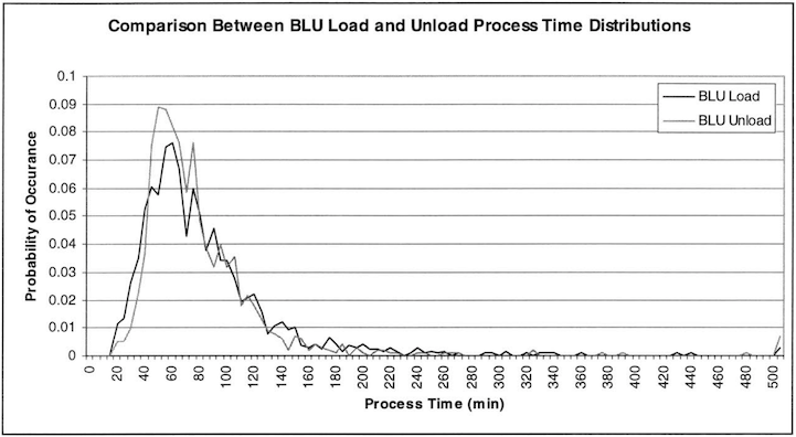
Because exponential/gamma distributions capture the true “long‐tail” behavior, LineLab automatically uses a gamma distribution to model process time variation.
Analyzing Data
You can just compute mean and standard deviation on any historical data using simple tools like Excel — even if the data points are gamma distributed. Statistical functions like STDEV work just the same on exponential or gamma distributed data.
- Standard deviation = mean × coefficient of variation (CV), as with all types of distributions.
- CV is a percentage (std / mean), broadly applicable across processes.
(As an aside: the so-called variance is CV squared.) So while standard deviation is a measure of time and commonly dependent on the process time average, the coefficient of variation is a percentage, which is broadly applicable.
Typical Coefficients of Variation (CV)
Even if your company has historical production data, you may have to review inputs if new processes may introduce new sources of variation. The following table contains typical values for the coefficient of variation (CV).
| Process / Industry | Coefficient of Variation | Source |
|---|---|---|
| Composite cure time | 1-22% | Mesogitis et al. 2016 |
| Resin transfer (composites) | 15-25% | Tifkitsis & Skordos 2020 |
| Aerospace composites production (AFP) | 10-30% | Nill 2018 |
| Spot welding | 14-112% | Kock 2008 |
| Lithography | 90-130% | Kock 2008 |
| Automotive: body shop | 10% | Fisher & Ittner 1999 |
| Brass piston discs, mid-size company | 50% | Millstein & Martinich 2014 |
| Semiconductor: burn-in | 50-90% | Terence 2001 |
| Wooden door manufacturing (manual) | 9-23% | Chen 2019 |
| Wooden door manufacturing (semi-automatic) | 2-20% | Chen 2019 |
| Healthcare (outpatient clinic) | 50-80% | Quiroz et al. 2018 |
If you're curious to find typical values for your industry: besides "process time variation", different engineers may refer to this concept as variation of the cycle time or process time variance, to name some examples.
Sources of High Process Time Variation
- Product variants with different geometry, processing characteristics, or component needs
- Processes with in-process adjustment needs, e.g. layup processes in composites
- Temporary sprints or "champion time" goals
- Varying energy & skill levels among workers
- Environmental conditions: humidity, temperature, lighting
Cost of Variation: Simple Example
In their book Manufacturing Systems Modeling and Analysis, G. Curry and R. Feldman analytically derive how a reduction in process time variability translates into a reduction in utilization (and thus an increase in the available capacity of a production system).
We can replicate the example in LineLab. The analytical approach is identical (and generally applicable to any type of distribution curve).
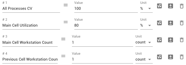
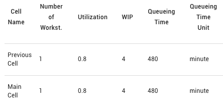
In the example, a process with a time of 2 hours has a coefficient of variation of 1 (i.e. 100%), and so does the arrival rate at the cell. The machine utilization is 80%. (We expose variables for cell utilization and workstation count to provide them as inputs.)
As in the example, a queueing time follows of 480 minutes, or 8 hours.
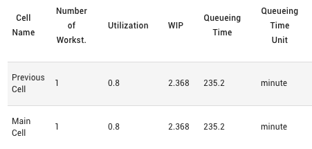
Now the process time variation is reduced, to show the difference. We will assume the coefficient of variation is cut by 30%.

As soon as we solve the changed model, we can see that queueing time drops by 51% from 480 (or 8 hrs) to 235.2 minutes (3.92 hrs):
This is of course a very simple example. In most production systems, WIP inventory comes at a big premium: more part carriers would be needed and more space to put them. And we know from Little's Law that there's a trade-off between flow time, WIP inventory and throughput.
So, to demonstrate what happens if inventory is fixed, we set the line WIP inventory to be the value it is at a CV of 70%.

We can now run a trade study to see how CV affects the throughput of the system:
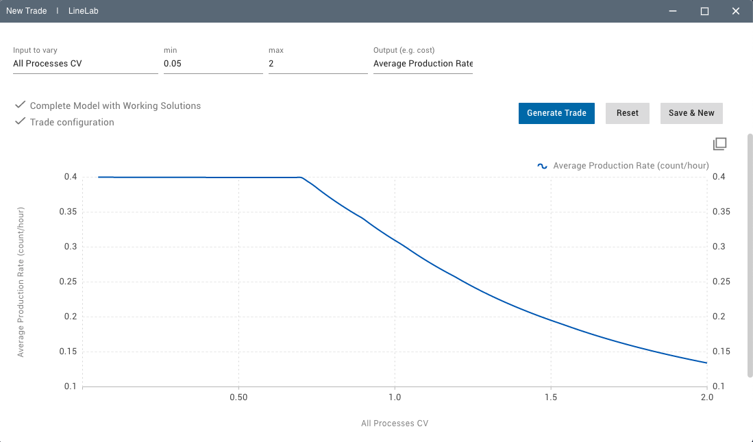
In the diagram, we can see that when the variation increases by half, the achievable throughput decreases by nearly 40%. However, the change is not linear.
We also observe that when the coefficient of variation is below where we fixed the system WIP (to the value LineLab calculated for maximizing rate), inventory is more than sufficient, so workstations are adequately utilized, and throughput is at its maximum. But with higher variation, the inventory limit leads to a decrease in machine utilization, resulting in a decrease in the achievable throughput. Because with higher variation, either more capacity or more inventory is needed; otherwise throughput decreases. That's why for a given system configuration, unless there's plenty of slack, any additional variation comes at a cost of the rate the system can handle.
So there is a very real cost to process time variation. It's a very non-linear effect and the relationships are complex, which is why it is so often misunderstood. But with the right tools, you can gain more of an intuition for it, and understand the often significant effects of process time variation on your unique production operations.